vcalib: differentiable calibration filters for RF-DETR under illumination shift

Table of contents

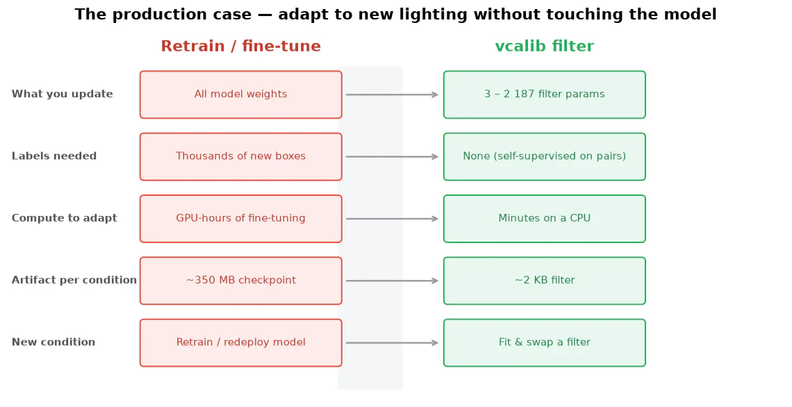
When the lighting changes, a detector trained under other conditions degrades. The textbook answer is to collect data, label it, retrain and redeploy. vcalib explores the cheap answer: keep the model frozen and fit, in minutes and without labels, a tiny filter that corrects the input.

The problem

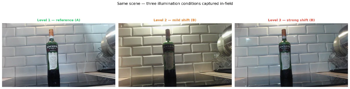
RF-DETR is a state-of-the-art real-time detector and, like almost any vision model, it is sensitive to illumination: dawn vs. dusk, indoor vs. overcast, a new camera, a new site. When the input distribution drifts away from the training one, detection quality drops. Retraining or fine-tuning is expensive, needs labels and is impractical on edge devices.

The same scene under three real lighting conditions — One scene captured under three real lighting conditions: exactly the kind of shift that moves a model’s internal features off-distribution.

The idea

Instead of adapting the model’s weights, vcalib adapts its input. A differentiable filter with between 3 and 2,187 parameters, depending on its type, transforms the shifted image before it reaches the frozen detector. It is the same economic logic that made LoRA and adapters win in NLP, applied to the input instead of the weights.

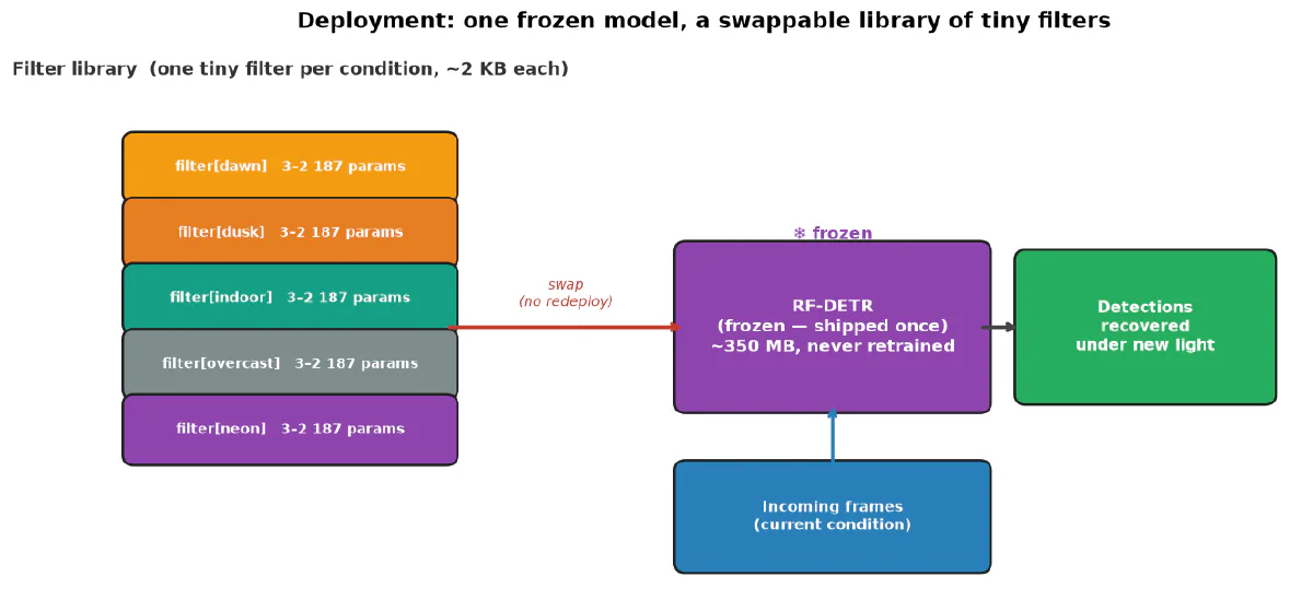
Cost of retraining vs. calibrating with vcalib — Retrain vs. calibrate: no labels, minutes on a CPU instead of GPU hours, and a ~2 KB artifact instead of a new checkpoint.

In deployment this becomes one frozen model plus a library of tiny filters, one per condition. Switching conditions means swapping a ~2 KB file: no retraining, no redeploy.

Deployment model: one frozen detector and swappable per-condition filters — Deployment model: one frozen detector and a swappable filter for each lighting condition.

How it works

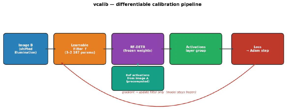
Calibration pipeline diagram — The filter is optimized against the frozen detector’s intermediate activations; the model never changes.

A few image pairs of the same scene are captured under the reference condition A and the shifted one B.
The filter is applied to B on the RGB tensor in [0, 1], before ImageNet normalization.
The frozen RF-DETR processes filter(B) and its intermediate activations are compared with the precomputed ones from A.
The loss is the mean relative activation distance over a layer group plus a regularization term. Adam updates only the filter parameters; about 100 steps per pair are enough.

Three design choices explain why this is not white balance under another name:

The signal is activations, not pixels. The objective is task-aware without any labels: the filter optimizes what the detector actually keys on, not human-perceived color. Classic linear corrections (white balance, affine) are included in the library and consistently underperform.
The layer group is a search axis. The set of RF-DETR layers feeding the loss is swept; the backbone’s multi-scale projector wins consistently.
Held-out validation as a guardrail. Every calibration is evaluated on unseen pairs, and an overfit gate (val/train ≥ 0.5) rejects degenerate configurations.

Results on real captured pairs

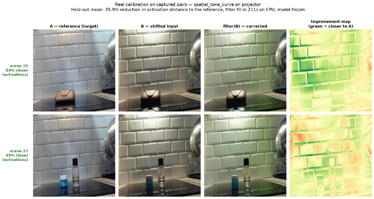
The winning filter (spatial_tone_curve, P=16, K=5, on projector) was trained on 24 real captured scenes and evaluated on 6 scenes held out entirely from training.

	Result
Mean activation-distance reduction (6 held-out scenes)	35.9%
Per-scene range	6.5% – 52.6%
Filter parameters	1,200
Fit time	~211 s on a laptop CPU (24 pairs, 60 epochs)
Model weights changed	0

Most of the recovery lands in the first 15 epochs.

Before and after calibration on real scenes — Left to right: reference A, the same scene under shifted lighting B, the corrected filter(B), and where the filter helped (green = closer to A). Real scenes the filter never saw during training.

Does it recover detection, not just activations?

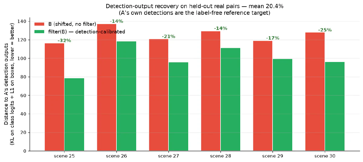
Activation distance is a proxy. What matters in production is whether the model detects the same things under the shift. Measured label-free, using the model’s own detections under A as the target, a filter calibrated against the detection objective pulls the outputs (logits and boxes) 20.4% closer to A, improving on all six scenes.

A clean lesson shows up here: what you optimize is what you recover. The activation-trained filter is great at activation recovery (35.9%) but only modestly recovers detection outputs (9.5%); calibrating against the detection objective doubles that figure.

Detection-output recovery per scene — Detection-output recovery on the 6 held-out scenes.

To turn this into a real mAP without the circularity of scoring the model against itself, the scenes are labeled with SAM3, a segmentation model independent of RF-DETR, and those boxes are used as pseudo-ground-truth. Class-agnostic COCO AP on the 6 held-out scenes (level_1 → level_2):

Arm	AP@[.5:.95]	AP50
A, reference	0.544	0.703
B, shifted	0.377	0.497
`filter(B)`, activation-trained	0.379	0.551
`filter(B)`, detection-trained	0.580	0.841

The detection-calibrated filter closes the entire A→B AP gap (121.5%) and on this set even scores above the reference on AP, AP50 and AP75 (0.614 → 0.619). The activation-trained one recovers barely 1% of AP.

Honest caveats. (1) This is SAM3 pseudo-ground-truth, not human annotation. (2) These are 6 test scenes: a few boxes move the numbers, so edging past the reference is real on this set but not a large-sample claim. (3) Recovery is cleanest at level_2; under the stronger level_3 shift the filter still recovers AP50 past the reference (0.756 vs 0.569 shifted and 0.703 reference) but trades high-IoU box precision, so strict AP goes flat-to-negative.

The 200-configuration sweep

Before the real pairs, a synthetic sweep of 200 configurations (filter × layer group × shift level) settled the design:

Layer group matters more than filter type. The backbone’s projector gives the strongest signal for every filter; results degrade from late to early layers.
Non-linear filters beat linear ones. Spatial tone curves and 3D LUTs capture the non-linear, per-channel character of a real illumination shift better than affine transforms.
The signal generalizes across shift levels. level_1 → level_3 gives slightly lower numbers with the same ranking.

Best sweep configuration: spatial_tone_curve (P=8, K=3) on projector, 30.7% reduction; lut_3d (N=9) reaches 29.6%.

What is proven and what is next

Proven. A tiny, label-free filter pulls a frozen detector’s internal representations back toward the reference condition (35.9% on real held-out pairs). The effect reaches the detection head (20.4%) and the mAP against independent pseudo-ground-truth. And it is cheap: thousands of parameters, minutes on a CPU, zero retraining.

Next milestone. mAP against human ground truth with a full retrain as the upper bound; confirming that one filter fitted once per environment holds across a whole stream of frames, not just isolated pairs; and an edge-deploy CLI that turns “fit and swap a filter” into a single command.

How it is built

Filter library: 18 parametric filters plus one neural filter, all sharing the interface Tensor[B,3,H,W] → Tensor[B,3,H,W], identity-initialized and end-to-end differentiable. From brightness_2param (2 parameters) to lut_3d (2,187) or neural_pixel, a per-pixel residual MLP.
Reproducible experimentation: YAML configs, run_experiments.py for sweeps, CSV results, pytest tests, and ruff plus mypy for linting.
Stack: Python 3.10+, PyTorch 2+, transformers, RF-DETR nano via LibreYOLO as a submodule, and uv as the package manager.

The code, sample data and full results live in the vcalib repository.